Introduction

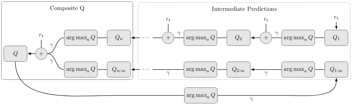
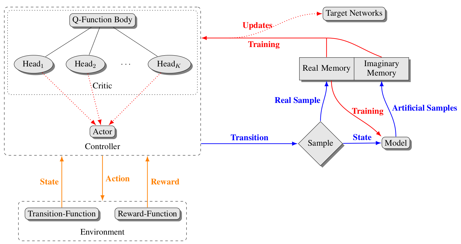
Popular Maximum Entropy Inverse Reinforcement Learning approaches require the computation of expected state visitation frequencies for the optimal policy under an estimate of the reward function. This usually requires intermediate value estimation in the inner loop of the algorithm, slowing down convergence considerably. In this work, we introduce a novel class of algorithms that only needs to solve the MDP underlying the demonstrated behavior once to recover the expert policy. This is possible through a formulation that exploits a probabilistic behavior assumption for the demonstrations within the structure of Q-learning. We propose Inverse Action-value Iteration which is able to fully recover an underlying reward of an external agent in closed-form analytically. We further provide an accompanying class of sampling-based variants which do not depend on a model of the environment. We show how to extend this class of algorithms to continuous state-spaces via function approximation and how to estimate a corresponding action-value function, leading to a policy as close as possible to the policy of the external agent, while optionally satisfying a list of predefined hard constraints. We evaluate the resulting algorithms called Inverse Action-value Iteration, Inverse Q-learning and Deep Inverse Q-learning on the Objectworld benchmark, showing a speedup of up to several orders of magnitude compared to (Deep) Max-Entropy algorithms. We further apply Deep Constrained Inverse Q-learning on the task of learning autonomous lane-changes in the open-source simulator SUMO achieving competent driving after training on data corresponding to 30 minutes of demonstrations. The scheme of Deep Constrained Inverse Q-learning can be seen in Fig. 1.

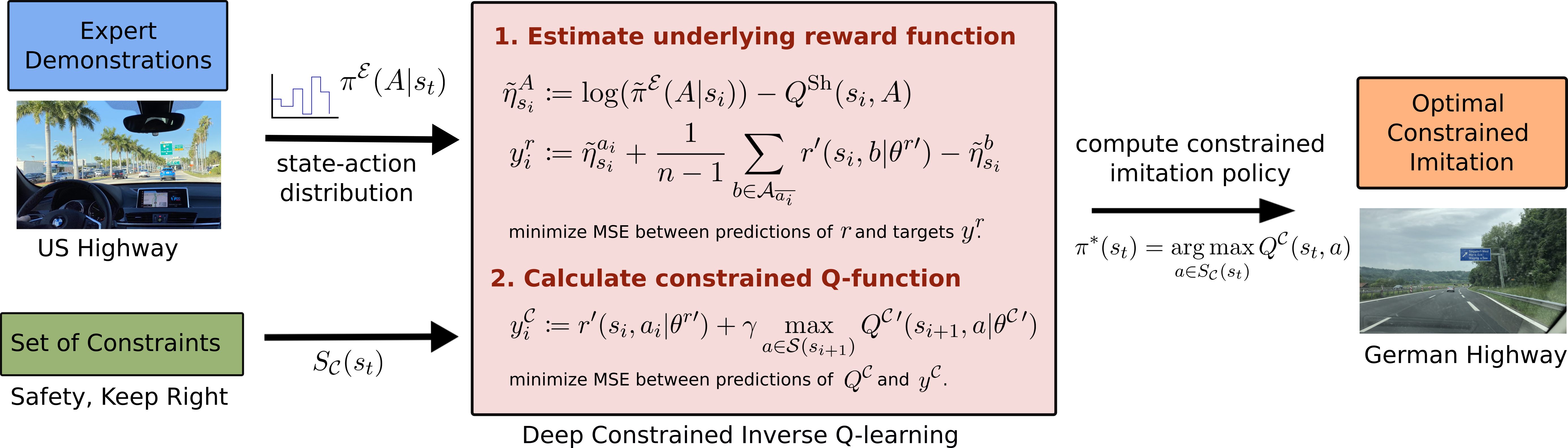
Fig. 1: Scheme of Deep Constrained Inverse Q-learning for the constrained transfer of unconstrained driving demonstrations, leading to optimal constrained imitation.

Technical Approach

Inverse Action-value Iteration

We start with the derivation of model-based Inverse Action-value Iteration (IAVI), where we first establish a relationship between Q-values of a state action-pair $(s,a)$ and the Q-values of all other actions in this state. We assume that the trajectories are collected by an agent following a stochastic policy with an underlying Boltzmann distribution according to its unknown optimal value function. For a given optimal action-value function $Q^*$, the corresponding distribution is: $$ \pi^\mathcal{E}(a|s) := \frac{\exp(Q^*(s, a))}{\sum_{A\in\mathcal{A}}\exp(Q^*(s, A))},$$ for all actions $a\in\mathcal{A}$. Rearranging gives: $$ \sum_{A\in\mathcal{A}}\exp(Q^*(s, A)) = \frac{\exp(Q^*(s, a))}{\pi^\mathcal{E}(a|s)} \text{ and } \exp(Q^*(s, a)) = \pi^\mathcal{E}(a|s)\sum_{A\in\mathcal{A}}\exp(Q^*(s, A)).$$ Denoting the set of actions excluding action $a$ as $\mathcal{A}_{\bar a}$, we can express the Q-values for an action $a$ in terms of Q-values for any action $b\in\mathcal{A}_{\bar a}$ in state $s$ and the probabilities for taking these actions: $$ \exp(Q^*(s, a)) =\pi^\mathcal{E}(a|s)\sum_{A\in\mathcal{A}}\exp(Q^*(s, A)) = \frac{\pi^\mathcal{E}(a|s)}{\pi^\mathcal{E}(b|s)}\exp(Q^*(s, b)).$$ Taking the log then leads to $$ Q^*(s, a)=Q^*(s, b) + \log(\pi^\mathcal{E}(a|s)) - \log(\pi^\mathcal{E}(b|s)).$$ Thus, we can relate the optimal value of action $a$ with the optimal values of all other actions in the same state by including the respective log-probabilities: $$(n-1) Q^*(s, a) = (n-1) \log(\pi^\mathcal{E}(a|s)) + \sum_{b\in\mathcal{A}_{\bar a}} Q^*(s,b) - \log(\pi^\mathcal{E}(b|s)).$$ The optimal action-values for state $s$ and action $a$ are composed of immediate reward $r(s, a)$ and the optimal action-value for the next state as given by the transition model, i.e. $Q^*(s, a)=r(s, a) + \gamma \max_{a'} \mathbf{E}_{s'\sim\mathcal{M}(s,a,s')}[Q^*(s', a')]$. Using this definition to replace the Q-values and defining the difference between the log-probability and the discounted value of the next state as: $$\eta_s^a =: \log(\pi^\mathcal{E}(a|s)) - \gamma \max_{a'}\mathbf{E}_{s'\sim\mathcal{M}(s,a,s')}[Q^*(s', a')],$$ we can then solve for the immediate reward: $$r(s, a) = \eta_s^a + \frac{1}{n-1} \sum_{b\in\mathcal{A}_{\bar a}} r(s, b) - \eta_s^b.$$ Formulating this equation for all actions $a_i \in \mathcal{A}$ results in a system of linear equations $\mathcal{X}_\mathcal{A}(s)\mathcal{R}_\mathcal{A}(s) = \mathcal{Y}_\mathcal{A}(s)$, with reward vector $\mathcal{R}_\mathcal{A}(s)$, coefficient matrix $\mathcal{X}_\mathcal{A}(s)$ and target vector $\mathcal{Y}_\mathcal{A}(s)$: $$ \begin{bmatrix} 1 & -\frac{1}{n-1} & \dots & -\frac{1}{n-1} \\ -\frac{1}{n-1} & 1 & \dots& -\frac{1}{n-1}\\ \vdots&\vdots & \ddots & \vdots\\ -\frac{1}{n-1} & -\frac{1}{n-1} & \dots & 1 \\ \end{bmatrix} \begin{bmatrix} r(s,a_1)\\ r(s,a_2)\\ \vdots\\ r(s,a_n)\\ \end{bmatrix} = \begin{bmatrix} \eta_s^{a_1} -\frac{1}{n-1}\sum_{b\in\mathcal{A}_{\overline{a_1}}} \eta_b^s\\ \eta_s^{a_2} -\frac{1}{n-1}\sum_{b\in\mathcal{A}_{\overline{a_2}}} \eta_b^s\\ \vdots\\ \eta_s^{a_n} -\frac{1}{n-1}\sum_{b\in\mathcal{A}_{\overline{a_n}}} \eta_b^s\\ \end{bmatrix}.$$

Tabular Inverse Q-learning

To relax the assumption of an existing transition model and action probabilities, we extend the Inverse Action-value Iteration to a sampling-based algorithm. For every transition $(s, a, s')$, we update the reward function using stochastic approximation: $$ r(s, a) \leftarrow (1 - \alpha_r) r(s,a)+ \alpha_r \left( \eta_s^a + \frac{1}{n-1} \sum_{b\in\mathcal{A}_{\bar a}} r(s, b) - \eta_s^b \right),$$ with learning rate $\alpha_r$. Additionally, we need a state-action visitation counter $\rho(s, a)$ for state-action pairs to calculate their respective log-probabilities: $\tilde{\pi}^\mathcal{E}(a|s) =: \rho(s, a) / \sum_{A \in \mathcal{A}} \rho(s, A).$ Therefore, we approximate $\eta_s^a$ by $\tilde{\eta}_s^a =: \log(\tilde{\pi}^\mathcal{E}(a|s)) - \gamma\max_{a'}\mathbf{E}_{s'\sim\mathcal{M}(s,a,s')}[Q^*(s', a')]. $ In order to avoid the need of a model $\mathcal{M}$, we evaluate all other actions via Shifted Q-functions as in Kalweit et al.: $$Q^\text{Sh}(s,a) =: \gamma\max_{a'}\mathbf{E}_{s'\sim\mathcal{M}(s,a,s')}[Q^*(s', a')],$$ i.e. $Q^\text{Sh}(s,a)$ skips the immediate reward for taking $a$ in $s$ and only considers the discounted Q-value of the next state $s'$ for the maximizing action $a'$. We then formalize $\tilde{\eta}_s^a$ as: $$\tilde{\eta}_s^a =:\log(\tilde{\pi}^\mathcal{E}(a|s)) - \gamma \max_{a'} \mathbf{E}_{s'\sim\mathcal{M}(s,a,s')}[Q^*(s', a')]= \log(\tilde{\pi}^\mathcal{E}(a|s)) - Q^{\text{Sh}}(s, a).$$ Combining this with the count-based approximation $\tilde{\pi}^\mathcal{E}(a|s)$ and updating $Q^\text{Sh}$, $r$, and $Q$ via stochastic approximation yields the model-free Tabular Inverse Q-learning algorithm (IQL).

Deep Inverse Q-learning

Deep Constrained Inverse Q-learning

Results

In Fig. 2 and Fig. 3, we evaluate the performance of IAVI, IQL and DIQL on the common IRL Objectworld benchmark and compare to MaxEnt IRL (closest to IAVI of all entropy-based IRL approaches) and Deep MaxEnt IRL (which is able to recover non-linear reward functions):

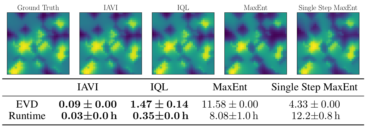
Fig. 2: Results for the Objectworld environment, given a data set with an action
distribution equivalent to the true optimal Boltzmann distribution.
Visualization of the true and learned state-value functions. Resulting expected
value difference and time needed until convergence, mean and standard
deviation over 5 training runs on a 3.00 GHz CPU.

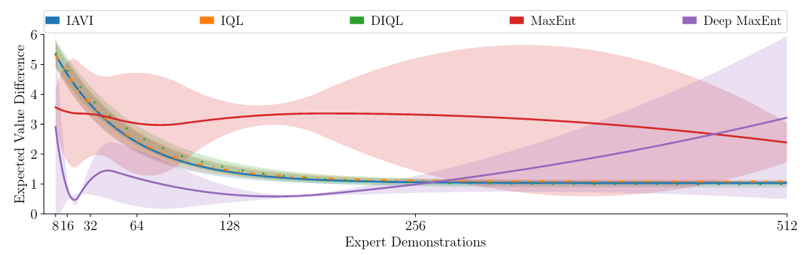
Fig. 3: Mean EVD and SD over 5 runs for different numbers of demonstrations
in Objectworld.

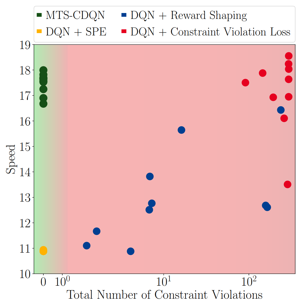
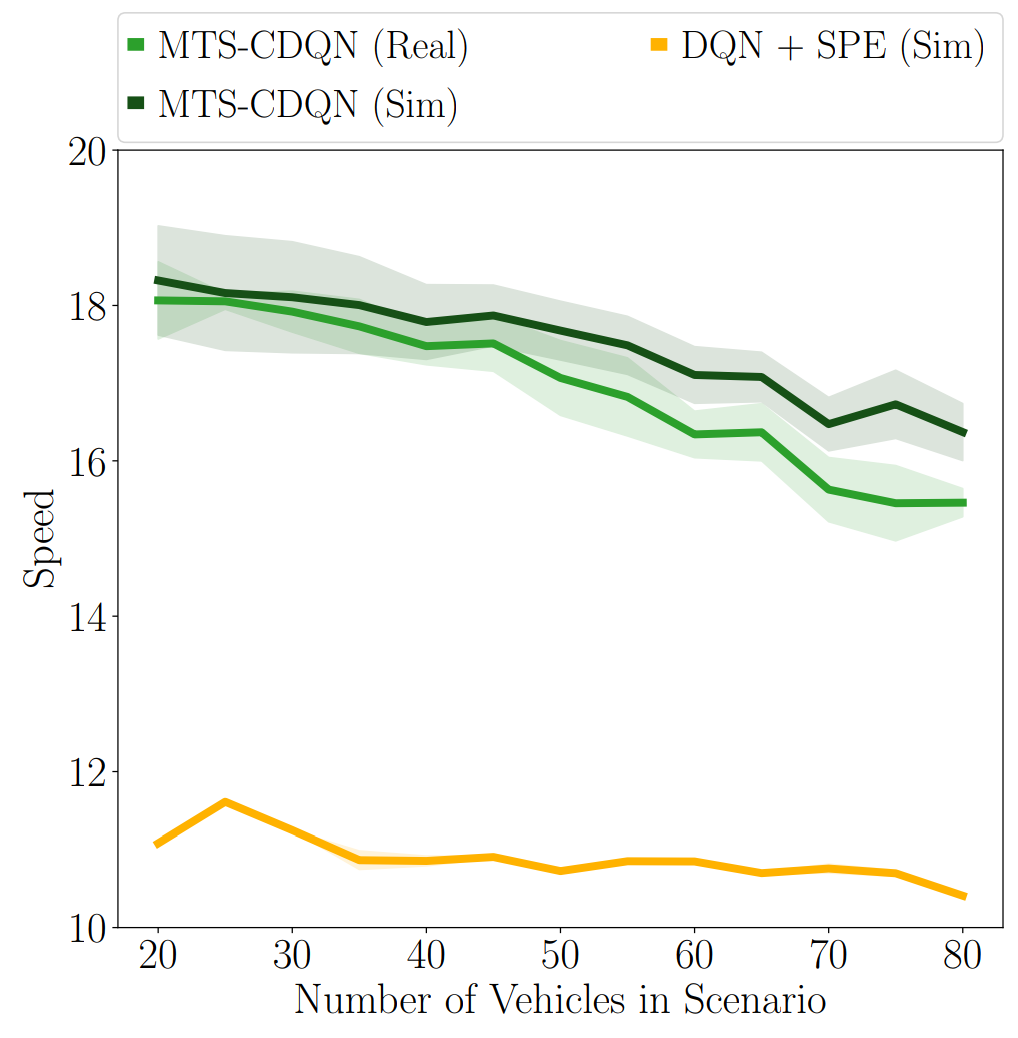
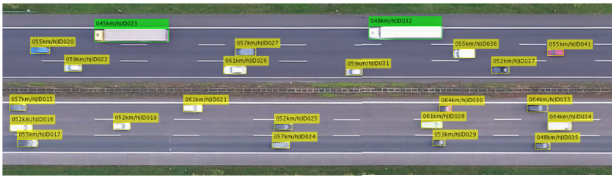
In Fig. 4 we show the potential of constrained imitation by DCIQL on a more complex highway scenario in the open-source traffic simulator SUMO:

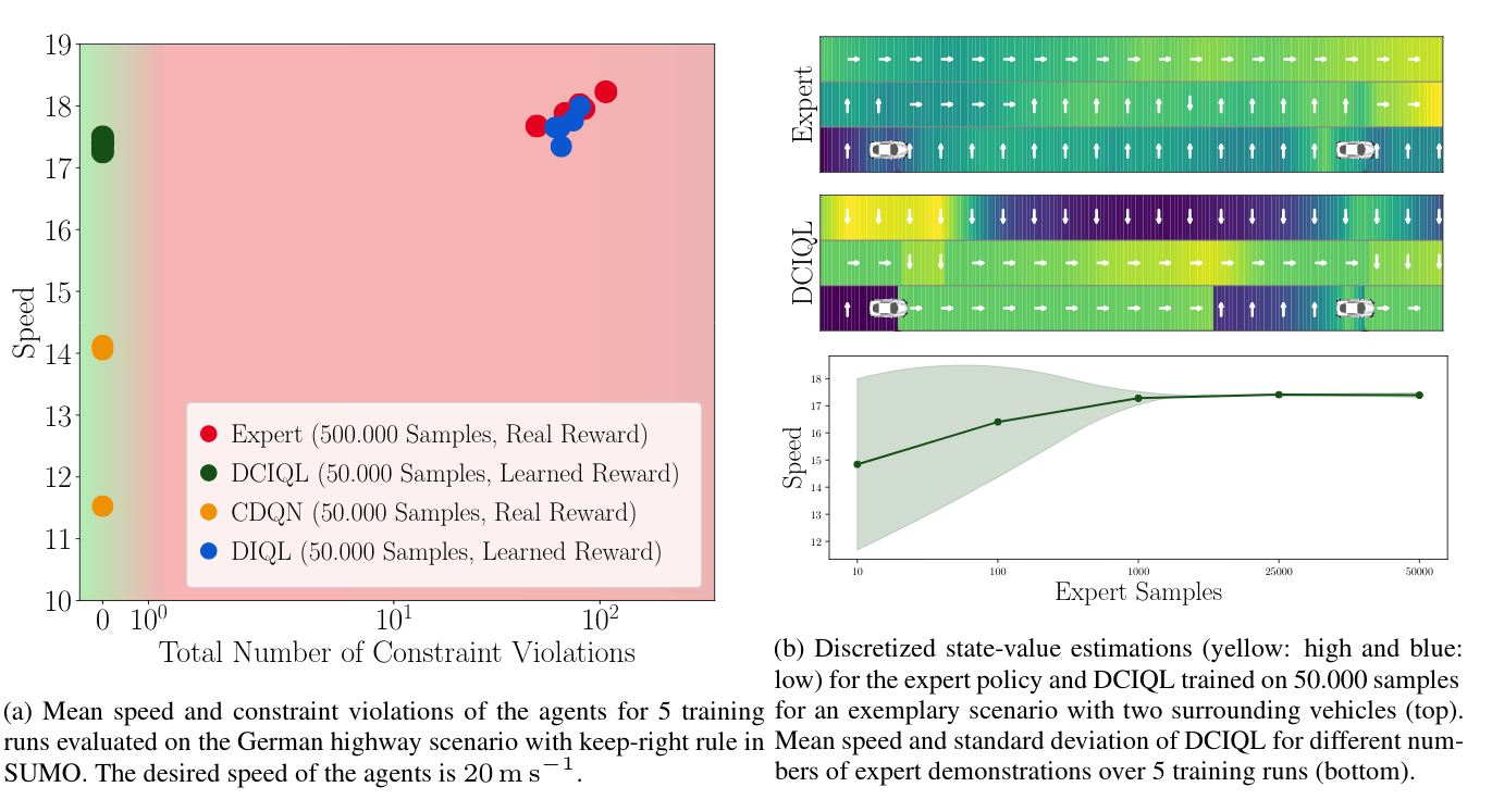
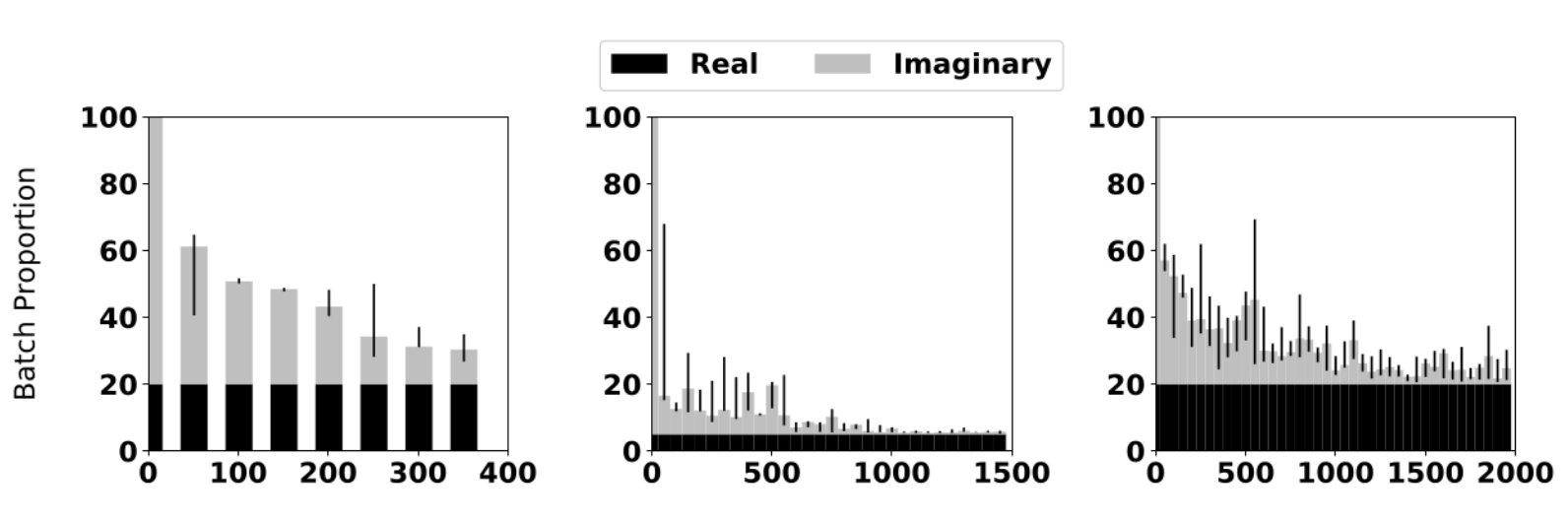
Fig. 4: Results for DCIQL in the autonomous driving task.

Demonstration

			
	@inproceedings{DBLP:conf/nips/KalweitHWB20,
	  author    = {Gabriel Kalweit and
	               Maria H{\"{u}}gle and
	               Moritz Werling and
	               Joschka Boedecker},
	  title     = {Deep Inverse Q-learning with Constraints},
	  booktitle = {Advances in Neural Information Processing Systems 33: Annual Conference
	               on Neural Information Processing Systems 2020, NeurIPS 2020, December
	               6-12, 2020, virtual},
	  year      = {2020},
	  url       = {https://proceedings.neurips.cc/paper/2020/hash/a4c42bfd5f5130ddf96e34a036c75e0a-Abstract.html},
	  timestamp = {Tue, 19 Jan 2021 15:57:00 +0100},
	  biburl    = {https://dblp.org/rec/conf/nips/KalweitHWB20.bib},
	  bibsource = {dblp computer science bibliography, https://dblp.org}
	}
							

Introduction

In the past few years, off-policy reinforcement learning methods have shown promising results in their application for robot control. Deep Q-learning, however, still suffers from poor data-efficiency and is susceptible to stochasticity in the environment or reward functions which is limiting with regard to real-world applications. We alleviate these problems by proposing two novel off-policy Temporal-Difference formulations: (1) Truncated Q-functions which represent the return for the first $n$ steps of a target-policy rollout w.r.t. the full action-value and (2) Shifted Q-functions, acting as the farsighted return after this truncated rollout. This decomposition allows us to optimize both parts with their individual learning rates, achieving significant learning speedup. We show that Truncated and Shifted Q-functions can be combined to the full return, leading to the Composite Q-learning algorithm. We show the efficacy of Composite Q-learning in the tabular case and compare Deep Composite Q-learning with TD3 and TD3($\Delta$), which we introduce as an off-policy variant of TD($\Delta$). Moreover, we show that Composite TD3 outperforms TD3 as well as state-of-the-art compositional Q-learning approaches significantly in terms of data-efficiency in multiple simulated robot tasks and that Composite Q-learning is robust to stochastic environments and reward functions. For an overview, see Fig. 1 below.

Fig. 1: Structure of Composite Q-learning. $Q_i$ denote the Truncated and $Q_{i:\infty}$ the Shifted Q-functions at step $i$. $Q$ is the complete Composite Q-function. Directed incoming edges yield the targets for the corresponding value-function. Edges denoted by $\gamma$ are discounted.

Technical Approach

Truncated Q-functions

In order to decompose the action-value into multiple truncated returns, assume that $n \ll (T-1)$ and that $(T-1-t)\mod n=0$ for task horizon $T$. We make use of the following observation: \begin{equation} \begin{split} Q^\pi(s_t, a_t)&=\mathbf{E}_{\pi,\mathcal{M}}\left[r_t+ \gamma r_{t+1} + \gamma^2 r_{t+2} + \gamma^3 r_{t+3} + \dots + \gamma^{T-1} r_{T-1}\right]\\ &=\mathbf{E}_{\pi,\mathcal{M}}\Biggl[\left({ \sum\limits_{j=t}^{t+n-1} \gamma^{j-t} r_j} \right) + \gamma^n \left({\sum\limits_{j=t+n}^{t+2n-1} \gamma^{j-(t+n)} r_j} \right)\\ &\qquad\qquad\qquad\qquad\qquad+ \dots +\gamma^{T-n} \left({ \sum\limits_{j=T-n}^{T-1} \gamma^{j-(T-n)} r_j} \right)\Biggr]. \end{split} \end{equation} That is, we can define the action-value as a combination of partial sums of length $n$. We can then define the Truncated Q-function as $Q^\pi_n(s_t, a_t)=\mathbf{E}_{\pi,\mathcal{M}}[\sum_{j=t}^{t+n-1}\gamma^{j-t}r_j]$, which we plug into the equation above: \begin{equation}\label{eq:trunc} \begin{split} Q^\pi(s_t, a_t)&=\mathbf{E}_{\pi,\mathcal{M}}[Q^\pi_n(s_t, a_t)+\gamma^n Q^\pi_n(s_{t+n}, a_{t+n})+\dots+\gamma^{T-n} Q^\pi_n(s_{T-n}, a_{T-n})].\\ \end{split} \end{equation} We approximate $Q^*_n(s_t, a_t)$ off-policy via consecutive bootstrapping. In order to limit the prediction to horizon $n$, we estimate $n$ different truncated value functions belonging to increasing horizons, with the first one estimating the immediate reward function. All consecutive value functions then bootstrap from the prediction of the preceding value function evaluating the target-policy of full return $Q$ for a fixed horizon. Analogous to vanilla Q-learning, the update procedure is given by: \begin{equation} \label{eq:truncatedqlearning} \begin{split} Q_1(s_t, a_t) &\leftarrow (1-\alpha_\text{Tr})Q_1(s_t, a_t) + \alpha_\text{Tr}r_t \text{ and }\\ Q_{i>1}(s_t, a_t) &\leftarrow (1-\alpha_\text{Tr})Q_i(s_t, a_t) + \alpha_\text{Tr}(r_t + \gamma Q_{i-1}(s_{t+1}, \argmax_a Q(s_{t+1}, a))), \end{split} \end{equation} with learning rate $\alpha_\text{Tr}$. Please note that in order to estimate the full return based on Truncated Q-functions alone, the dynamics model would be needed to get $s_{t+c\cdot n}$ of a rollout starting in $s_t$. In the following, we describe an approach to achieve an estimation of the full return model-free.

Shifted Q-functions

To get an estimation for the remainder of the rollout $Q_{n:\infty}^\pi=\mathbf{E}_{\pi,\mathcal{M}}[\gamma^n Q(s_{t+n}, a_{t+n})]$ after $n$ steps, we use a consecutive bootstrapping formulation of the Q-prediction as a means to skip the first $n$ rewards of a target-policy rollout: \begin{equation} \begin{split} Q_{1:\infty}(s_t, a_t) &\leftarrow (1-\alpha_\text{Sh})Q_{1:\infty}(s_t, a_t) + \alpha_\text{Sh}(\gamma \max_a Q(s_{t+1}, a)) \text{ and}\\ Q_{(i>1):\infty}(s_t, a_t) &\leftarrow (1-\alpha_\text{Sh}) Q_{i:\infty}(s_t, a_t) + \alpha_\text{Sh}(\gamma Q_{(i-1):\infty}(s_{t+1}, \argmax_a Q(s_{t+1}, a))), \end{split} \end{equation} with learning rate $\alpha_\text{Sh}$. We hypothesize that Shifted Q-functions allow for higher learning rates, since they only have to account for the variance of the underlying dynamics and not of the immediate reward function, as opposed to conventional value functions.

Composition

Following the definitions of Truncated and Shifted Q-functions, we can compose the full return: \begin{equation} \begin{split} Q(s_t, a_t) \leftarrow (1-\alpha_Q)Q(s_t, a_t) + \alpha_Q(r_t + \gamma (&Q_n(s_{t+1}, \argmax_a Q(s_{t+1}, a))\\ &+ Q_{n:\infty}(s_{t+1}, \argmax_a Q(s_{t+1}, a)))). \end{split} \end{equation} The incorporation of truncated returns breaks down the time scale of the long-term prediction by the Shifted Q-function. We call this algorithm Composite Q-learning. Please note that Composite Q-learning is equivalent to Q-learning when setting $\alpha_\text{Tr}=\alpha_\text{Sh}=\alpha_Q$. However, a notable advantage is that Composite Q-learning offers an independent optimization for the different learning rates corresponding to different temporal horizons.

Deep Composite Q-learning

We apply Composite Q-learning within TD3. Let $Q^{\text{Tr}}(\cdot, \cdot|\theta^{{\text{Tr}}})$ denote a function approximator with parameters $\theta^{{\text{Tr}}}$ and $n$ outputs, subsequently called heads, estimating Truncated Q-functions $Q_i$. Each output $Q^{\text{Tr}}_i$ bootstraps from the prediction of the preceding head, with the first approximating the immediate reward function. The targets are therefore given by: \begin{equation}\label{eq:trunctarget0} y^{\text{Tr}}_{j, 1} = r_j \text{ and } y^{\text{Tr}}_{j, i>1} = r_j + \gamma Q_{i-1}^{\text{Tr}\prime}(s_{j+1}, \mu^{\prime}(s_{j+1}|\theta^{\mu\prime})|\theta^{{\text{Tr}\prime}}), \end{equation} where $\mu^{\prime}$ corresponds to the target-actor maximizing the full Q-value and $Q_{i-1}^{\text{Tr}\prime}$ the output of the respective Q-target-network. That is, $Q^{\text{Tr}}$ represents evaluations of $\mu$ at different stages of truncation and $y^{\text{Tr}}_{j, i< n}$ serve as intermediate predictions to get $y^{\text{Tr}}_{j, n}$. We then only use $Q^\text{Tr}_n$, which implements the full $n$-step return, as the first part of the composition of the Q-target, but not the $Q^\text{Tr}_{i< n}$ values. The second part of the composition is represented by the Shifted Q-function. Let $Q^{\text{Sh}}(\cdot, \cdot|\theta^{{\text{Sh}}})$ denote the function approximator estimating the Shifted Q-functions $Q_{i:\infty}^\pi$ by $n$ different outputs, parameterized by $\theta^{{\text{Sh}}}$. We can shift the Q-prediction by bootstrapping without taking the immediate reward into account, so as to skip the first $n$ rewards of a target-policy rollout. The Shifted Q-targets for heads $Q^{\text{Sh}}_i$ therefore become: \begin{equation}\label{eq:shiftedtarget0} y_{j, 1}^\text{Sh}=\gamma Q^\prime(s_{j+1}, \mu^\prime(s_{j+1}|\theta^{\mu\prime})|\theta^{Q\prime}) \text{ and } y_{j, i>1}^\text{Sh}=\gamma Q^{\text{Sh}\prime}_{i-1}(s_{j+1}, \mu^\prime(s_{j+1}|\theta^{\mu\prime})|\theta^{{\text{Sh}\prime}}). \end{equation} In the function approximation setting, we can thus define the Composite Q-target as: \begin{equation}\label{eq:qtarget} y^Q_j=r_j + \gamma (Q^{\text{Tr}\prime}_n(s_{j+1}, \mu^\prime(s_{j+1}|\theta^{\mu\prime})|\theta^{{\text{Tr}\prime}}) + Q^{\text{Sh}\prime}_n(s_{j+1}, \mu^\prime(s_{j+1}|\theta^{\mu\prime})|\theta^{{\text{Sh}\prime}})), \end{equation} approximated by $Q(\cdot, \cdot|\theta^Q)$ with parameters $\theta^Q$.

Results

Vanilla Reward

In Fig. 2 and 3, we show the data-efficiency of Tabular Composite Q-learning and Shifted and Truncated Q-functions for a deterministic chain MDP of arbitrary horizon.

Fig. 2: (a) Deterministic chain MDP.
(b) Results of Composite Q-learning in the MDP shown in (a) with a horizon of 20.

Fig. 3: (a) Results of Composite and Shifted Q-learning with different learning rates for the
Shifted Q-function. (b) Results of Composite Q-learning with different learning rates
for the Truncated Q-function.

Noisy Reward

Fig. 4 shows the data-efficiency of Tabular Composite Q-learning for a stochastic chain MDP of arbitrary horizon.

Fig. 4: (a) Stochastic chain MDP.
(b) Results for Composite Q-learning for the MDP shown in (a).

Lastly, we compare in Fig. 6 Composite TD3, TD3($\Delta$) and TD3 at default setting and with high learning rate (HL) in multiple MuJoCo benchmarks shown in Fig 5.

Fig. 5: MuJoCo environments.

Fig. 6: Mean performance and half a standard deviation over 8 runs for (left) Walker2d-v2,
(middle) Hopper-v2 and (right) Humanoid-v2 with uniform noise
on the reward function as in Romoff et al., 2019.

			
@misc{kalweit2019composite,
	title={Composite Q-learning: Multi-scale Q-function Decomposition
	and Separable Optimization},
	author={Gabriel Kalweit and Maria Huegle and Joschka Boedecker},
	year={2019},
	eprint={1909.13518},
	archivePrefix={arXiv},
	primaryClass={cs.LG}
}
							

Introduction

In many real world applications, reinforcement learning agents have to optimize multiple objectives while following certain rules or satisfying a list of constraints. Classical methods based on reward shaping, i.e. a weighted combination of different objectives in the reward signal, or Lagrangian methods, including constraints in the loss function, have no guarantees that the agent satisfies the constraints at all points in time and lack in interpretability. When a discrete policy is extracted from an action-value function, safe actions can be ensured by restricting the action space at maximization, but can lead to sub-optimal solutions among feasible alternatives. In this work, we propose Multi Time-scale Constrained DQN, a novel algorithm restricting the action space directly in the Q-update to learn the optimal Q-function for the constrained MDP and the corresponding safe policy. In addition to single-step constraints referring only to the next action, we introduce a formulation for approximate multi-step constraints under the current target policy based on truncated value-functions to enhance interpretability. We compare our algorithm to reward shaping and Lagrangian methods in the application of high-level decision making in autonomous driving, considering constraints for safety, keeping right and comfort. We train our agent in the open-source simulator SUMO and on the real HighD data set. For an intuition, see Fig. 1 below.

Fig. 1: In this MDP, state $s_6$ is marked as unsafe. Assume a safety check with a horizon of two time steps and that the initial state is $s_0$. Unconstrained Q-learning (red) chooses the unsafe path leading to $s_9$ with a return of $+2$ and Safe Policy Extraction (blue) after Q-learning leads to a safe path to state $s_{10}$ with a return of $+0.5$. Multi Time-scale Constrained Q-learning (green) chooses the safe path to $s_{11}$ with a return of $+1$.

Theoretical Background

Reinforcement Learning

In a reinforcement learning setting, an agent interacts with an environment, which is typically modeled as an MDP $\langle\mathcal{S}, \mathcal{A}, \mathcal{P}, r, \gamma\rangle$. The agent is following policy $\pi : \mathcal{S} \rightarrow \mathcal{A}$ in some state $s_t$, applying a discrete action $a_t \sim \pi$ to reach a successor state $s_{t+1}\sim\mathcal{P}$ according to a transition model $\mathcal{P}$. In every discrete time step $t$, the agent receives reward $r_{t}$ for selecting action $a_t$ in state $s_t$. The goal of the agent is to maximize the expectation of the discounted long-term return $\mathbf{E}_{a_i\sim\pi, s_{i>t}\sim\mathcal{P}}[R(s_t)] = \mathbf{E}_{a_i\sim\pi, s_{i>t}\sim\mathcal{P}}[\sum_{i\geq t} \gamma^{i-t}r_i]$, where $\gamma \in [0, 1]$ is the discount factor. The action-value function $Q^\pi(s_t,a_t)=\mathbf{E}_{a_{i>t}\sim\pi, s_{i>t}\sim\mathcal{P}}[R(s_t)|a_t]$ represents the value of following a policy $\pi$ after applying action $a_t$. The optimal policy can be inferred from the optimal action-value function $Q^*(s_t, a_t) = \max_{\pi} Q^{\pi}(s, a)$ by maximization.

Constrained Markov Decision Processes (CMDP)

We consider a CMDP $\langle\mathcal{S}, \mathcal{A}, \mathcal{P}, r, \gamma, \mathcal{C}\rangle$, with constraint set $\mathcal{C} = \mathcal{C}^a \cup \mathcal{C}^\pi$, where the set of signals $ \mathcal{C}^a = \{ c_i:\mathcal{S} \times \mathcal{A} \rightarrow \mathbb{R} | 1 \le i \le N \}$ for single-step constraints only depend on the current state and action. We define the set of safe actions for a single-step constraint $c_i \in \mathcal{C}^a$ as $S_{c_i}(s_t) = \{a \in \mathcal{A} | \ c_i(s_t, a) \le \beta_{c_i} \}$. The set $ \mathcal{C}^\pi = \{ \mathcal{J}^\pi_{H_i,i} :S \times A \rightarrow \mathbb{R} | \ 1 \le i \le M \}$ consists of multi-step constraint signals $\mathcal{J}^\pi_{H_i,i}$ with horizon $H_i$ which are dependent on policy $\pi$. The set of expected safe actions of a multi-step constraint $\mathcal{J}^\pi_{H_i,i}\in\mathcal{C}^\pi$ is defined as $S^\pi_{\mathcal{J}^\pi_{H_i,i}}(s_t) = \{a \in \mathcal{A} | \ \mathcal{J}^\pi_{H_i,i}(s_t, a) \le \beta_{\mathcal{J}^\pi_{H_i,i}} \}$. We define $S_\mathcal{C}(s_t)$ as the intersection of all safe sets.

Safe Policy Extraction

Given an action-value function $Q$ and a set of constraints $\mathcal{C}$, we can extract the optimal safe policy $\pi$ w.r.t. $Q$ by $\pi(s_t) = \argmax_{a\in S_\mathcal{C}(s_t)}Q(s_t, a)$. We call this method Safe Policy Extraction (SPE).

Technical Approach

While common constraints are only dependent on the current decision step, it can be crucial to represent the effect of the current policy of the agent for a longer time scale. Typically, long-term dependencies on constraints are represented by the expected sum of discounted or average constraint signals $j_i$, i.e. $\mathcal{J}^\pi(s_t, a_t) = \mathbf{E}_{a_{i>t}\sim\pi, s_{i>t}\sim\mathcal{P}}[J(s_t)|a_t] = \mathbf{E}_{a_{i>t}\sim\pi, s_{i>t}\sim\mathcal{P}}[\sum_{i\geq t} \gamma^{i-t}j_i]$. Instead, we only consider the next $H$ steps: $\mathcal{J}^\pi_H(s_t, a_t) = \mathbf{E}_{a_{i>t}\sim\pi, s_{i>t}\sim\mathcal{P}}[J_H(s_t)] = \mathbf{E}_{a_{i>t}\sim\pi, s_{i>t}\sim\mathcal{P}}[\sum_{i\geq t}^{t + H} j_i]$. Due to the fixed horizon $H$, discounting is not needed, which leads to more interpretable constraints. We apply the formulation of truncated value-functions to predict the truncated constraint-values. We first estimate the immediate constraint-value and then follow a consecutive bootstrapping scheme to get to the estimation of the full horizon $H$. The update rules for constraint-values $\mathcal{J}^\pi_h$ are: \begin{align*} \mathcal{J}^\pi_{1}(s_t, a_t)\leftarrow&(1-\alpha_{\mathcal{J}}) \mathcal{J}^\pi_1(s_t, a_t)+\alpha_{\mathcal{J}} j_t \text{ and}\\ \mathcal{J}^\pi_{h>1}(s_t, a_t)\leftarrow&(1-{\alpha_{\mathcal{J}}}) \mathcal{J}^\pi_h(s_t, a_t)+\alpha_{\mathcal{J}} (j_t + \mathcal{J}^\pi_{h-1}(s_{t+1}, \argmax_{a\in S_{\mathcal{C}}(s_{t+1})} Q(s_{t+1}, a))), \end{align*} with constraint-specific learning rate $\alpha_{\mathcal{J}}$. To cope with infinite state-spaces, we jointly estimate $\mathcal{J}^{\pi}_h|_{1\leq h\leq H}$ with function approximator $\mathcal{J}(\cdot, \cdot|\theta^\mathcal{J})$, parameterized by $\theta^\mathcal{J}$. We extend the Q-learning update to use a set of constraints $\mathcal{C} = \mathcal{C}^a \cup \mathcal{C}^\pi$ with corresponding safe action set $S_{\mathcal{C}}(s_{t+1})$: $$Q^\mathcal{C}(s_t, a_t) \leftarrow (1 - \alpha) Q^\mathcal{C}(s_t, a_t) + \alpha (r + \gamma \mathop{\max_{\ a \in S_{\mathcal{C}}(s_{t+1})}} Q^\mathcal{C}(s_{t+1}, a)).$$ The optimal deterministic constrained policy $\pi^* \in \Pi_{S_{\mathcal{C}}}$ is: $$\pi^*(s_t) = \mathop{\argmax_{a \in S_{\mathcal{C}}(s_t) }} Q^\mathcal{C}(s_{t}, a).$$ We refer to this algorithm as Multi Time-scale Constrained DQN (MTS-CDQN).

Results

In Fig. 2, we show performance and constraint violations of MTS-CDQN, DQN+SPE, DQN + Reward Shaping and DQN + Constraint Violation Loss. In Fig. 3, we then show the performance of MTS-CDQN trained on the real HighD data set. As can be seen, the approach is very robust to real data which we visualize in Fig. 4.

Fig. 2
Fig. 3
Fig. 2: Results for MTS-CDQN in the autonomous driving task.
Fig. 3: Results for MTS-CDQN trained on the real HighD data set.

Fig. 4: Visualization of the HighD data set.

Demonstration

			
@misc{kalweit2020interpretable,
  title={Interpretable Multi Time-scale Constraints in Model-free 
  Deep Reinforcement Learning for Autonomous Driving},
  author={Gabriel Kalweit and Maria Huegle and Moritz Werling and Joschka Boedecker},
  year={2020},
  eprint={2003.09398},
  archivePrefix={arXiv},
  primaryClass={cs.LG}
}
							

Introduction

Continuous control of high-dimensional systems can be achieved by current reinforcement learning methods such as the Deep Deterministic Policy Gradient algorithm (DDPG) and its extensions, but needs a significant amount of data samples. For real-world systems, this can be an obstacle since excessive data collection can be expensive, tedious or lead to physical damage. The main incentive of this work is to keep the advantages of model-free $Q$-learning while minimizing real-world interaction by the employment of a dynamics model learned in parallel. To counteract adverse effects of imaginary rollouts with an inaccurate model, a notion of uncertainty is introduced, to make use of artificial data only in cases of high uncertainty. We evaluate our approach on three simulated robot tasks and achieve faster learning by up to factor 15 in comparison to vanilla DDPG with multiple updates. For an overview, see Fig. 1 below.

Fig. 1: Structure of MA-BDDPG.

Technical Approach

Model-assisted DDPG

We approach the problem with a deterministic model and learn to predict the state change: $\mathcal{M}^\Delta: \mathcal{S}\times\mathcal{A}\mapsto\Delta_\mathcal{S}$. In each time step, the agent collects a real sample $s_t$, which is the starting point for $B$ imaginary rollouts of specified depth $D$. For each step, the action $a_{bd}$ is selected based on the current real policy and random noise. For training, target values, loss and target update are equivalent to DDPG. Since actor and critic are updated on imaginary samples, for those updates it comes down to \begin{equation} \label{eq:lossimaginedsamples} \hat{\mathcal{L}}(\theta^Q)=\frac{1}{n}\sum\limits_i (\hat{y}_i-Q(\hat{s}_i, a_i|\theta^Q))^2, \end{equation} where target values $\hat{y}_i$ are defined as $\hat{y}_i=r(\hat{s}_i, a_i) + \gamma Q'(\hat{s}_{i+1}, \mu'(\hat{s}_{i+1}|\theta^{\mu'})|\theta^{Q'}) $ and the occuring states $ \hat{s}_i = \mathcal{M}^\Delta(\hat{s}_{i-1}, a_{i-1})+\hat{s}_{i-1}$. The critic is updated on $U_r$ real batches and $U_i$ imaginary batches and, thus, gets gradients from both loss functions in each cycle. We call this algorithm Model-assisted DDPG (MA-DDPG).

Including Uncertainty

In order to incorporate the uncertainty estimate and to still be able to adapt to continuous action domains, the Bootstrapped DQN architecture is extended to follow the actor-critic scheme of DDPG. The $Q$-function approximator $Q_{1:K}(\cdot, \cdot|\theta^Q)$ is defined to be a deep neural network with parameters $\theta^Q$ composed of an optional single shared body and $K$ independent network heads $Q_k$. Analogously to DDPG and MA-DDPG, the target values get computed via slowly updated target networks $Q'_{1:K}$ and $\mu'$. When the agent receives a new transition, it generates a random mask $\mathbf{m}_t = (m^1, m^2, \dots, m^K)_t$ with $m^i\sim \mathbf{P}$, for some probability distribution $\mathbf{P}$. In the experiments, each element of the mask is drawn according to a Bernoulli distribution with sharing probability $p$. This ensures that a sample is only seen by some subset of the heads and, hence, $K$ bootstrapped samples are created. The $K$ heads are then trained on their respective samples. First, the different target values for the $K$ heads are calulated,$y_t^{Q_{1:K}} \leftarrow r_t + \gamma Q'_{1:K}(s_{t+1},\mu'(s_{t+1}|\theta^{\mu'})|\theta^{Q_{1:K}'})$, and then the critic gets updated on the combined loss, \begin{equation} \mathcal{L}(\theta^{Q_{1:K}}) = \sum\limits_k\frac{1}{n_k}\sum\limits_im^k_i(y^k_i-Q^k(s_i,a_i|\theta^{Q_k}))^2, \end{equation} where $n_k=\sum\limits_i\delta_{m_i^k\neq0}$ and $\delta$ is the Dirac delta function. Note that the masks modify the loss, so as to redirect the gradients only to the corresponding heads. The parameters $\theta^\mu$ of single-network actor $\mu$ are then updated according to the mean of all respective updates of all heads, \begin{equation} \nabla_{\theta^\mu}R\leftarrow \frac{1}{K}\sum\limits_k\frac{1}{n}\sum\limits_i\nabla_aQ^k(s_i,a|\theta^{Q^k})|_{a=\mu(s_i)}\nabla_{\theta^\mu}\mu(s_i|\theta^\mu). \end{equation} After updating critic and actor, the weights of the target networks $Q'_{1:K}$ and $\mu'$ get shifted towards the current weights by $\tau\in(0,1]$, analogously to DDPG. Based on the distribution over $Q$-functions, the agent can then estimate its uncertainty by its variance.

Limiting Model Usage

A simple way to limit the use of imagination proportional to the current uncertainty is to transform the uncertainty measure to a probability distribution and to induce a biased coin flip. The result of the coin flip then determines whether to train on an imaginary batch or not. The variance of an agent could be task specific. On the other hand, the measure should not depend on prior knowledge over the variance. In order to circumvent this necessity, we put the uncertainty into context of the maximum variance seen so far. Formally, we define the probability of learning on minibatch $b$ from the imaginary replay buffer $\mathcal{I}$ as $\mathbf{P}[b\subset\mathcal{I}]=\hat{\sigma}^2_{e+1}=\bar{\sigma}^2_e/\max_E\bar{\sigma}^2_{E< e}$ in episode $e$, where $\bar{\sigma}^2_e$ denotes the mean variance in $e$. This restricts the mean variance ratio in $[0, 1]$ and can be interpreted as follows: if it is unknown whether a value of variance is high or not, the maximum value is a rational reference point. Hence, this underlying probability distribution yields a dimensionless measure of uncertainty and should decrease over time when the different heads of the critic converge.

Results

Fig. 2 depicts the final results of MA-BDDPG compared to DDPG with default setting and multiple updates per collected sample. As can be seen, MA-BDDPG yields an improved data-efficiency of up to factor 15. The amount of artificial samples, however, decreases over time along with the variance within the Q-ensemble, as shown in Fig. 3.

Fig. 2: Comparison of MA-BDDPG and DDPG with default setting
and multiple updates per time step. MA-BDDPG
is up to 15 times more data-efficient.
Fig. 3: Ratio of real and artificial transitions during training. The use of virtual samples
decreases over time.

Demonstration

			
@InProceedings{pmlr-v78-kalweit17a,
title = {Uncertainty-driven Imagination for Continuous Deep Reinforcement Learning},
author = {Gabriel Kalweit and Joschka Boedecker},
booktitle =  {Proceedings of the 1st Annual Conference on Robot Learning},
pages = {195--206},
year = {2017},
editor = {Sergey Levine and Vincent Vanhoucke and Ken Goldberg},
volume = {78},
series = {Proceedings of Machine Learning Research},
month = {13--15 Nov},
publisher =  {PMLR},
pdf =  {http://proceedings.mlr.press/v78/kalweit17a/kalweit17a.pdf},
url =  {http://proceedings.mlr.press/v78/kalweit17a.html},
}